Baokun Huang, Yu Wang, Shuhao Zhou, Xinzhang Li
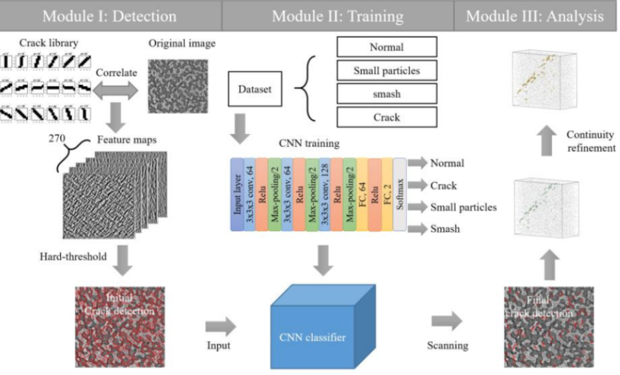
Fig1[1]: image from “Automated damage analysis of a bio-cellular material via feature-based learning in X-ray tomography, Ziling Wu, Ting Yang, Baokun Huang, Han Liu, Yu Wang, Hongwei Lou, Ling Li, Yunhui Zhu”
The paper analyzed the images of X-ray CT sea urchin skeleton structure, by detecting the cracks and small particles. The dataset of the paper comes from a X-ray tomography reconstruction. The whole structure is split to 2160 layers of tiff images. But these images are noisy and the cracks are small, scattering in images. The flowchart above shows how they find the crack.
In the module 1, the paper generates 433 pieces of cracks. Once these cracks are generated, they are used to do a correlation with the original image to find the potential points in the original images. The idea of this approach is to reduce the calculation of the networks and make results be more accurate.
In the module 2, the paper build a 15 layers CNN network to classify these features. And the network is trained with cropped 32x32x1 images. These images are pre labeled by crack and non crack or small particles and normal features.
In the module 3, since the images of the structure are continuous, the paper use the adjoint results to do the test.
It is impossible to get X-ray scan of sea urchin. Theresore, we tried our best to search online open database and identify the most close one with our paper.
In the paper we selected, there are two folders in database. One folder contains crack, while another folder contains non-crack.
Therefore, the database we search for should have the same folder settings. We found several public database including Pavement crack detection[1], CrackForest dataset[2], and some other public open database. Eventually, we decided to use SDNET2018[3], because it contains three types of images, each type contains two folders, cracks and non cracks, and the background was less noisy. The data size is 256x256x3, jpg files.
One difference between paper’s database and our database was that our database was one or more large cracks in the image. However, the origin database was several small crack scattered in the images. This difference could make a difference in our future steps.
The evaluation method we used is from “Automatic Pavement Crack Detection Based on Structured Prediction with the Convolutional Neural Network”, written by Zhun Fan, Senior Member, IEEE, Yuming Wu, Jiewei Lu, and Wenji Li. We will produce two files before the evaluation process, PositiveResults.mat and NegativeResults.mat. We will evaluate these two files by using the following evaluation equation.
Pr = TP / (TP + FP)
Re = TP / (TP + FN)
F1 = (2 x Pr x Re) / (Pr + Re) [3]
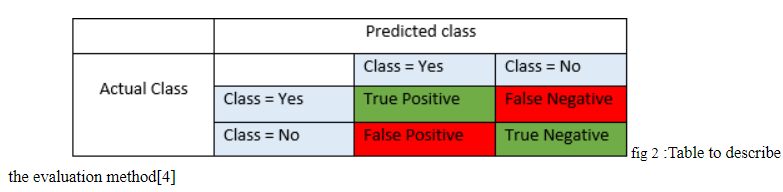
Pr (precision), Re (recall), F1 (F1 score), TP (number of true positive), FP (number of false positive), FN (number of false negative).
Pr tells us the ratio of the correct true prediction to the total number of predictions which predicted as true. If Pr has high rate then we know most of the true prediction is correct.
Re tells us the ratio of the correct true prediction to the total number of all class with yes in actual class in table above.
F1 Score is the weighted average of Precision and Recall. Therefore, this score takes both false positives and false negatives into account.[4]
Due to limited time, we setted up three steps before we started execution:
(1)Use network to classify the crack and non-crack This step was used to proof that we can use this network to classify the data we needed. The result was expected to be bad and we will fix that later.
(2)Adjust the ratio between crack and non-crack in train database. This step was learnt from paper. After adjust the ratio between crack and non crack, we expected to get a better result.
(3)After finding the best ratio, we crop new training database by imageJ Fiji, label them by crack and non crack.
(4)Correlation with the ourself generate crack, if the point is higher than 0.75, we will identify it as a possible point. We will test the possible point in our trained network.
We will go through the results in different steps in the following.
Procedure:
The data we get is pre-labeled. At first we want to see if the network from paper can correctly classify this dataset as it is given. The work we are going to do in this part is just using the network from the paper train partial dataset. And test the some part of other part dataset. The result is shown in the below.
Detail: We get 1000 cracks and 1000 non cracks for training. The rest data are used for testing.
Results Evaluation
TP: 655 FP: 5385 FN: 389
Pr = 0.108 Re= 0.627 F1= 0.184
Findings
Since all three measurements are not high, we want to try other approaches to improve our results.
Procedure:
Since the results from the simple training doesn’t work very well, we want to try the adjust ratio between crack and non crack. The idea comes from a paper we read. We want to see, within different ratio of cracks and non cracks, can we improve our results or not.
The reason behind that raio of crack and non cracks matters is that the number of crack patches and the number non cracks are imbalanced in a single image. This will cause a problem that, for instance, if we have 5 cracks in 100 training data, even if the network detected all these be non cracks, the accuracy will be 95%. To solve this problem, try different ratio is a solution.
In the paper, it concludes 1:3 for a database and 1:2 for another, so that I realized that different database may have different best ratio. We want to find the best ratio of this database.
We plan to test 1:1, 1:2, 1:3 and 1:4 to see the different. Since a single test is time consuming and the size of images,we cannot do more tests. The rest part of this approach is the same as the last one.
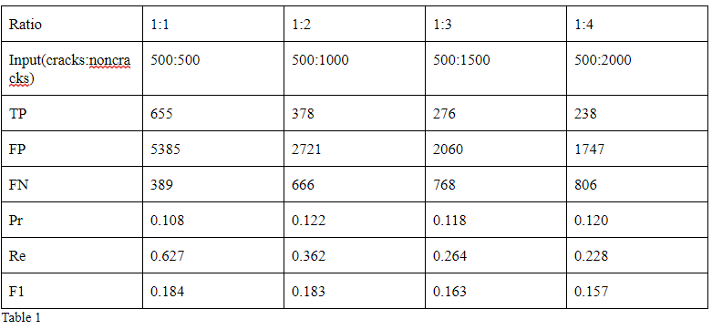
Plot Graph Compare different ratio
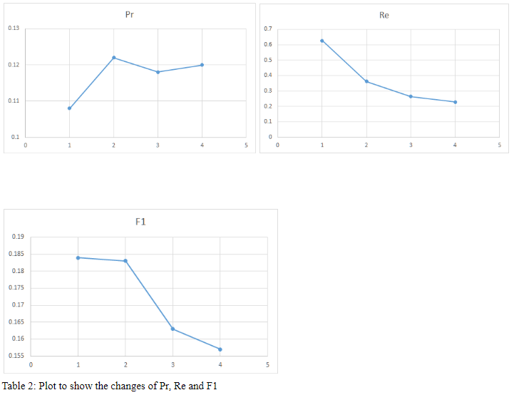
Analyze the plot and conclude
Based on fig above, we can see that change in ratio can affect the value of recall and F1 score. Smaller ratio will have higher recall and F1 score. Higher ratio will have lower recall and F1 score. Thus, ratio 1:1 would be better than other ratios.
For the precision, we can’t have an accurate answer on the relation between precision and ratio. However, we can assume ratio doesn’t change precision because the four precision values vary in a range of 0.
There are some changes by different ratio but this approach doesn’t improve our results.
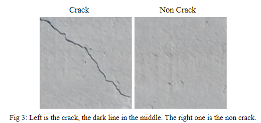
We crop the cracks and non cracks by ImageJ, a software that can easily label the features by pointing. After the pointing, we crop the according 32x32x3 images, change to grayscales and normalize them to be 32x32x1 and store them for the next step. These two images generated from the cropping process. The left is the crack. The right is the non crack. Both are not normalized nor graysscelaed . There is a light crack on the right side of the crack images. And the non crack image have some noise.
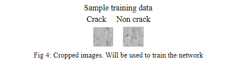
We crop 500 cracks and 500 non cracks. We trained them in the network after we normalized them. The following is the results of network testing..
Results Evaluation
TP: 238 FP: 69 FN: 806
Pr: 0.775 Re: 0.228 F1: 0.352
Analyze result
Compare to step 2, step 3 have higher accuracy.
With the smaller images the training process is faster.
With the normalization preprocess, the accuracy is higher than step 2 and 1
This results confirm that with the same techs in the paper will improve the accuracy. But we cannot confirm that this accuracy is high enough for the following approaches.
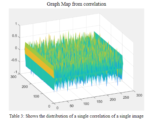
Correlation is a big part in this paper. Since they mentioned that without correction there many errors. We generate 433 cracks as they do and try to find the high risk point in the image. The following image is the sample map results from the correlation. The z-axis shows how the 32x32x1 images around this point is similar to the cracks we generated. We choose the value > 0.75 to be the high risk. The following graph comes from the a single correlation. The yellow part are positive and the blue part are negative. The higher the more similar, the lower the less similar.
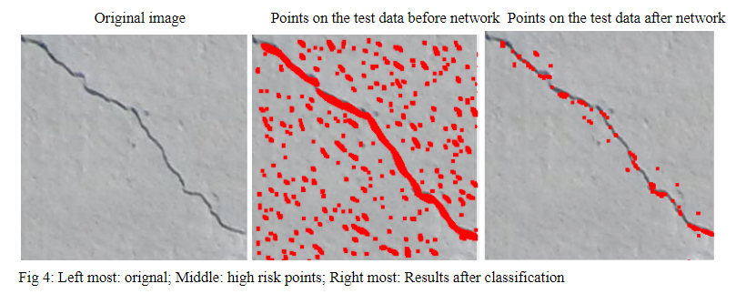
Procedure & Reuslts:
Next step is to crop the same size of images as the ones we trained in the network so as to classify the results. The following three images show the result. The original image is directly from the dataset. The second images is the images that contain the red point which comes from the correlation process. These high risk points are the points we will test in this step. These red points form a middle line which is the crack we want to highlight. But there are some noise high risk points around it. The goal at this step is to use the network to get rid of these line and keep the middle line as much as possible. After we use the network to classify all the 32x32x1 images located at high risk points, we remove most of the incorrected points and leave some of points on the crack. You can see the result in the third image. The third one is last result. It is clearly depict the crack location, although the high risk pint are getting less. The noise are totally removed. The reason that the red points are not centered on the crack is that we test the images with a 32x32x1 cropping images so that the test images from red points near crack will also contain part of crack. These crack will cause the images be classified as crack.
The results can be clearly detected, we think we have reproduced the paper.
The data in the paper is a 3D structure that has some continuous crack which we don't, because we could not find any 3D structure scan images on the website. So we abandon the module 3, which is used to test the continuity of crack in different layers.
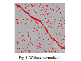
Based on our several approaches, we can conclude that the ratio of the cracks and noncracks doesn’t work for this dataset. But the normalization will do, since we can compare the fig 4 and fig 5. That the images resulting from unnormalized preprocessing training doesn’t remove much noncrack points but the normalized does. So may be, the normalized ratio test will work. But we don't have time to do that. And since the by comparing our results with the result in the paper can clearly describe the cracks, we can conclude we successfully reproduce the paper result.
[1] https://github.com/fyangneil/pavement-crack-detection
[2] https://github.com/cuilimeng/CrackForest-dataset
[3] Fan, Zhun, et al. Automatic Pavement Crack Detection Based on Structured Prediction with the Convolutional Neural Network . 1 Feb. 2018.
[4] “Accuracy, Precision, Recall & F1 Score: Interpretation of Performance Measures.” Exsilio Blog, 11 Nov. 2016, blog.exsilio.com/all/accuracy-precision-recall-f1-score-interpretation-of-performance-measures/.
[5] Wu, Ziling, et al. “Automated Damage Analysis of a Bio-Cellular Material via Feature-Based Learning in X-Ray Tomography.”
[6] Fan, Zhun, et al. “Automatic Pavement Crack Detection Based on Structured Prediction with the Convolutional Neural Network.” arxiv.org/abs/1802.02208v1.